Peak fitting

Peaks

Fit up to ten Gaussian, Lorentzian, Voigt or Resonance peaks — the shapes that spectral lines and driven oscillators most often take in nature.

01The peak options

There are four peak-fitting options:

• Gaussian
• Lorentzian
• Voigt
• Resonance

With the exception of the two Resonance options — which each fit a single peak — every type offers a maximum of 10 peaks to fit the data. The initial estimate of each peak’s position is picked with the Pick Peaks cursor tool in the Context Menu.

Once a peak is fitted, the right-hand pane shows the fitting coefficients in terms of the amplitude a, the width w, the peak position p and any constant offset c. The amplitude is measured with respect to that offset; the position is the centre of the peak; and the width w is the peak’s full width at half maximum (FWHM), also measured relative to the offset. For the Gaussian, Lorentzian and Voigt shapes the fitted w equals the FWHM exactly.

02The peak types

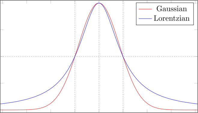
A comparison of a Gaussian and a Lorentzian profile, scaled to the same height and width.

The Voigt profile is a linear combination** of these two, where the ratio of their contributions can be adjusted from 0.1 to 0.9. When you select the Voigt option and choose the number of peaks, you are prompted to modify the Voigt ratio or keep the current value. A setting of 0.1 is nearly pure Lorentzian and 0.9 nearly pure Gaussian, with the default of 0.5 giving an equal contribution from each.

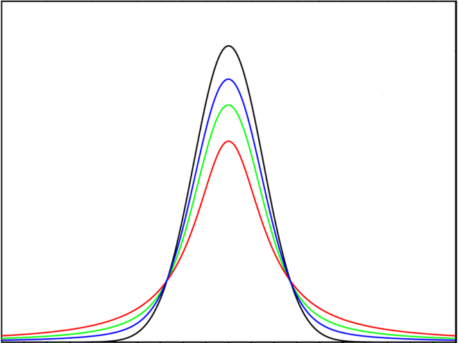
A series of Voigt profiles, from Gaussian to Lorentzian.

03Why these peak shapes?

These shapes occur commonly in nature. Take a spectral line such as the emission of a laser beam: while a perfect laser might be expected to emit a single frequency — a narrow line — in practice that line is broadened by physical processes. Doppler broadening gives a Gaussian profile, while collision broadening (or pressure broadening) and lifetime broadening give a Lorentzian profile. Spectral lines of many origins (lasers, atomic transitions and so on) often show shapes broadened by some combination of these processes.

04The Resonance peaks

CFTool offers two Resonance options, both designed to fit damped, driven harmonic-oscillator data of the kind found in mechanical or electrical systems:

• Amplitude Resonance — the mechanical resonator’s amplitude response.
• Power Resonance — its power response, i.e. the amplitude squared.

Damped resonance curves are not symmetrical, and CFTool fits assuming the typical asymmetry of a mechanical system. Both options use the coefficients amplitude a, width w, resonant angular frequency ω₀ and constant offset c — here ω₀ takes the place of the peak position p used by the other peak types.

05Peak-fitting tips

CFTool can fit up to 10 peaks on a graph simultaneously — but they will all share a common baseline. If that holds for your data, fine; if your peaks sit on a changing baseline, you may find it easier to fit one or two peaks close together and place the fitting limits just outside them. The plot below needed only two peaks to make this fit.

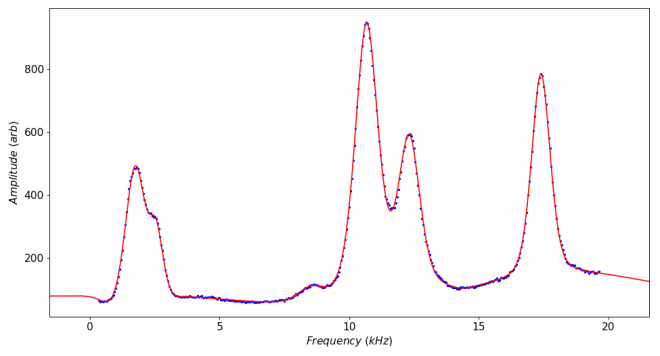
There is also a trick for changing baselines: choose some “peaks” on the line between the main peaks to make the curve follow the baseline. This can work well, but you must be careful which set of coefficients corresponds to the main peaks of interest. The plot below uses this technique, but required all 10 peaks to define the shape.