Reading results
The Parameter Sweep tool holds the structure fixed, varies one parameter across a range, solves at every point, and plots a figure of merit against it — sheet resistance, sheet carrier density, peak field or ionised fraction. It is the quickest way to see how one design choice trades off, without editing and re-running by hand.
01Opening the tool
Open it from File → Parameter Sweep…. It works on the structure currently in the main window, so build or open a device first, then open the tool. Each run sweeps that structure, changing one parameter at a time and leaving everything else — the other layers, the boundary and the temperature — exactly as you set it.
If you change the structure in the main window while the tool is open, press Refresh from structure to pick up the change before running again. The layer list at the top of the window is re-read at the same time.
02Describing a sweep
The window lists the current structure’s layers at the top, numbered from the surface, so you can see which index is which. A graded layer shows both ends of the grade as surface→substrate (for example a doping reading 1e18→1e16), so a graded field is not mistaken for a uniform one. Below the table is a single command line. A sweep is described by a short set of flags:
- –param thickness|doping|x|temperature — the parameter to sweep. A doping sweep varies whichever dopant the layer already carries in the table, keeping its type, so the layer must be set to a single dopant (n or p) first. The x sweep varies a ternary layer’s mole fraction — the aluminium fraction for AlGaAs, the indium fraction for InGaAs, and so on — and applies only to an alloy layer. Temperature is a whole-structure sweep — it changes the temperature of the entire solve, not one layer.
- –layer N — which layer to vary, by the index shown in the table (0 is the surface layer). It is required for a layer parameter. For a temperature sweep it is optional: temperature is applied to the whole structure regardless, and –layer then just selects which layer the per-layer figures of merit report on (layer 0 if you omit it).
- –start X –stop Y — the range, in the parameter’s own units (nm for thickness, cm⁻³ for doping, a percentage 0–100 for the mole fraction x (the same units as the layer table, so 30 means x = 0.30), kelvin for temperature).
- –num K — how many points across the range (11 if omitted).
- –log — space the points logarithmically rather than linearly; the natural choice for a doping sweep, which usually spans decades.
- –dx nm — override the mesh spacing for the sweep, the same setting as Mesh Spacing in the main window. A coarser mesh makes a long sweep quicker; a finer one is steadier at low temperature.
For example, –layer 0 –param doping –start 1e16 –stop 1e19 –num 12 –log sweeps the surface layer’s doping across three decades in twelve logarithmic steps, and –param temperature –start 50 –stop 400 –num 12 sweeps the whole structure’s temperature from 50 to 400 K. Press Run (or Enter) to start. A progress bar tracks the solves and can be cancelled at any point; each point is a full solve, so a long sweep takes a few seconds. A mistyped command is reported below the box rather than acted on.
A composition sweep holds the strain fixed. Each ternary in the materials database carries its properties as curves in the mole fraction x, fitted for one strain state on a named substrate — the built-in InGaAs, for instance, is pseudomorphic on GaAs, with relaxed InGaAs a separate entry. An x sweep slides along those fixed curves; it does not recompute the strain, the critical thickness, relaxation, or the polarisation charge in a nitride as the composition changes. A narrow sweep near the composition you actually grow is reliable; a wide one drifts away from reality, because in a real film the strain and the band offsets move with x. Treat a broad composition sweep as indicative, and do not read the strained-to-relaxed transition off it — that is a change of material, not a point on the curve.
03Choosing what to plot
A single sweep computes several figures of merit at once. The Plot: selector, beside Refresh from structure, lists the ones the sweep produced; choosing a different one re-draws the stored data instantly, without solving again. The figures are:
- Sheet resistance (Ω/sq) — the lateral sheet resistance of the whole stack, the same parallel-conduction figure described in Sheet Resistance and Transport. This is the default.
- Sheet electron density and Sheet hole density (cm⁻²) — the free carriers integrated through the whole structure.
- Sheet electron density (swept layer) and Sheet hole density (swept layer) — the same, but for the one layer named by –layer.
- Peak electric field (V/cm) — the largest field magnitude anywhere in the structure.
- Ionised fraction (swept layer) — the fraction of the swept layer’s net doping that is actually ionised, measured in the layer’s interior so surface depletion does not skew it. This is the activation quantity: it is near one when the dopants are fully active and falls as they freeze out. It is meaningful only with partial ionisation selected (see Temperature and Ionisation); with full ionisation it is pinned at one by definition.
04Reading the result
The plot draws the selected figure against the swept parameter. The x-axis is logarithmic when you passed –log, and the figures that span decades — sheet resistance and the sheet densities — are drawn on a logarithmic y-axis. The legend can be dragged out of the way if it covers the curve. A line below the command box reports the outcome, and carries any note about the sweep — for instance that a graded layer moved only at its surface, or that a temperature sweep was run with full ionisation, where freeze-out is switched off.
The Data table… button opens the numbers behind the plot in a separate window, with one column per figure of merit, which stays in step as you re-run. Save Plot (PNG)… and Save Data (CSV)… write the figure and the full table to files of your choosing.
05A worked example: dopants freezing out
The clearest thing a temperature sweep shows is incomplete ionisation made measurable. Take a single p-type GaAs layer doped to 1×1017 cm−3, choose partial ionisation, and sweep the temperature from 300 K down to 50 K. Plot the ionised fraction and the sheet resistance together:
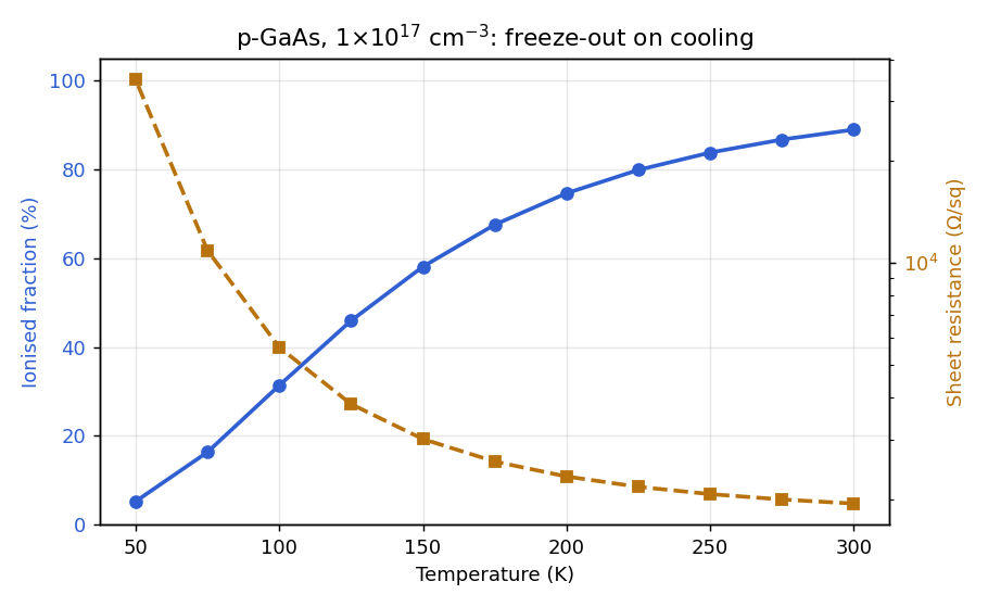
At room temperature nearly every acceptor has given up its hole, so the ionised fraction sits close to one and the sheet resistance is at its floor. Cooling reduces the thermal energy available to lift holes off the acceptors, so a growing fraction of them freeze back onto the dopant — the layer is not fully activated any more. Because sheet resistance is set by the free-carrier count, it rises in step: here from about 1.9 kΩ/sq at 300 K to about 35 kΩ/sq at 50 K. The two curves are the same physics read two ways — one as the cause (carriers leaving the bands), one as the measurable consequence (resistance rising).
This is why the ionised-fraction figure is meaningful only under partial ionisation. Full ionisation forces every dopant to stay active at every temperature, so the ionised fraction would be a flat line at one and the sheet resistance would barely move — the tool says so if you run a temperature sweep that way.
One variable, other conditions held. A sweep varies a single parameter and holds everything else fixed. It therefore answers “how does this figure change with this parameter, under these conditions,” not how the device behaves once several things change together. Each point is a complete solution, so the result is exactly what the main window would give for that one value — a sweep is just many of those runs collected onto one axis. Sweeping a layer that is graded on the swept quantity moves only its surface-side value; the tool says so when that happens.

